Upper Limits on the Stochastic Gravitational-Wave Background from Advanced LIGO's First Observing Run
- plots from the publication
Contents
- Figure 1 - Narrowband estimator for Omega_GW
- Figure 2 - 95% confidence region in Omega_alpha-alpha plane
- Figure 3 - Limits and models across many decades in frequency
- Figure 4 - 95% confidence region in average chirp mass - local rate plane
- Figure 5 - Spectra from binary black holes for different mass distributions
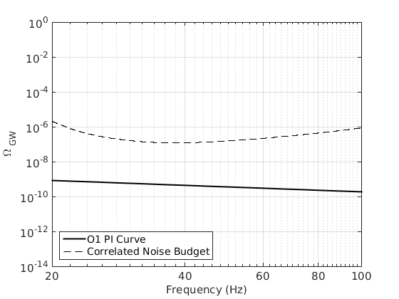
- Supplement Figure 1 - Magnetic correlated noise budget
Figure 1 - Narrowband estimator for Omega_GW
h=figure;

% load in data
tmp=load('figure1.dat');
freq=tmp(:,1);
Omega0=tmp(:,2);
two_sigma=tmp(:,3);

%set font size
set(0,'defaultaxesfontsize',18);

%parameters for plotting
fmin=20;
fmax=85.75; % band containing 99% of sensitivity
Omega_range=3.5e-5/0.68^2;

% plot Omega0 vs f
plot(freq, Omega0,'color',[.5 .5 .5],'LineWidth',2)
hold on

% plot +/- 2 sigma error bars
plot(freq,two_sigma,'k','LineWidth',2)
plot(freq,-two_sigma,'k','LineWidth',2)
hold off

% make axes
grid on
xlabel('Frequency (Hz)')
ylabel('\Omega_0')
axis([fmin fmax -Omega_range Omega_range])

print(gcf,'-depsc','figure1.eps')
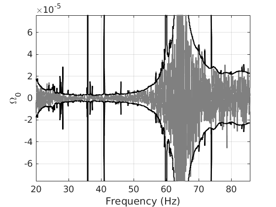
Figure 2 - 95% confidence region in Omega_alpha-alpha plane
figure;

%load contours
tmp=load('figure2_initial.dat');
a_init=tmp(:,1);
Om_init=tmp(:,2);

tmp=load('figure2_O1.dat');
a_O1=tmp(:,1);
Om_O1=tmp(:,2);

tmp=load('figure2_design.dat');
a_des=tmp(:,1);
Om_des=tmp(:,2);


%set up figure
gg = axes;
set(gg,'FontSize',18);

% plot Initial LIGO-Virgo contour
semilogy(a_init,Om_init,'k','linewidth',2)
hold on

% plot O1 contour
semilogy(a_O1,Om_O1,'b','linewidth',3)

% plot Design contour
semilogy(a_des,Om_des,'linestyle','--','linewidth',2,'color',[0.5 0.5 0.5])

% set up grid and legend
grid on
xlabel('\alpha','FontSize',18);
ylabel('\Omega_{\alpha}','FontSize',18);
legend('Initial LIGO-Virgo','aLIGO O1','Design','Location','NorthEast')

axis([-5 5 1e-12 1e-3])
ax=gca;
set(ax,'XTick',[-5:5]);
set(ax,'YTick',[1e-12 1e-11 1e-10 1e-9 1e-8 1e-7 1e-6 1e-5 1e-4 1e-3]);

grid minor
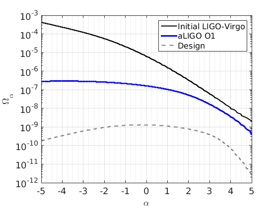
Figure 3 - Limits and models across many decades in frequency
figure('units','normalized','position',[0 0 1 0.4])

% parameters for font size
hh = axes;
set(hh,'FontSize',15)

fs=15; %font size for labels
lw=1.5; %line width for curves
green=[0 0.8 0]; %RGB vector for plotting dark green


% Plots are made in this order: PI curves (Initial LV, O1, Design, H1-H2,
% Indirect Limits, CMB, LISA), Pulsar Limit, Earth's normal modes, BNS, BBH,
% slow-roll inflation

% Initial LIGO-Virgo PI curve
tmp = load('PICurve_InitialLV.dat');
freq=tmp(:,1);
Om=tmp(:,2);

loglog(freq,Om,'k','linewidth',lw);
hold on

text(1e-3,1e-3,'Initial LIGO-Virgo','FontSize',fs,'Color','k')


% O1 PI Curve
tmp = load('PICurve_O1.dat');
freq=tmp(:,1);
Om=tmp(:,2);

loglog(freq,Om,'b','linewidth',lw);

text(1e-1,1e-5,'aLIGO O1','FontSize',fs,'Color','b')


% Design PI Curve
tmp = load('PICurve_design.dat');
freq=tmp(:,1);
Om=tmp(:,2);

loglog(freq,Om,'Color',[0.5,0.5,0.5],'LineWidth',lw,'LineStyle','--');

text(7e2,5e-6,'Design','FontSize',fs,'Color',[0.5 0.5 0.5]);


% H1H2 PI Curve
tmp=load('PICurve_H1H2.dat');

freq=tmp(:,1);
Om=tmp(:,2);

loglog(freq,Om,'Color','r','linewidth',lw)

text(2e3,7.7e-4,'H1-H2','Color','r','FontSize',fs)


% Indirect Limits
% Phys. Rev. X 6, 011035
tmp=load('figure3_IndirectLimits.dat');
freq=tmp(:,1);
Om=tmp(:,2);

loglog(freq,Om,'Color',[0.4 0.4 0.4],'LineStyle','-','linewidth',lw)
text(1e-9,1e-5,'Indirect Limits','FontSize',fs,'Color',[0.4 0.4 0.4])


% CMB
% Phys. Rev. X 6, 011035
tmp=load('figure3_CMB_LowL.dat');

freq=tmp(:,1);
Om=tmp(:,2) * 2;  % Convert 1 to 2 sigma

loglog(freq,Om,'Color','m','LineWidth',lw)
text(2e-16,1e-13,'CMB','FontSize',fs,'color','m')

% LISA
% Phys.Rev. D88 (2013) no.12, 124032
tmp=load('PICurve_LISA.dat');

freq=tmp(:,1);
Om=tmp(:,2);

loglog(freq,Om,'Color',[1 0 0],'LineWidth',lw,'linestyle','--')
text(1e-4,1e-11,'LISA','FontSize',fs,'color',[1 0 0])


% Pulsar limit
% Phys. Rev. X 6, 011035
freq=2.8e-9;
Om=2.291035e-10;

loglog(freq,Om,'color',green,'Marker','p','MarkerSize',5,'markerfacecolor',green)

text(1.5e-9,5e-11,'Pulsar','FontSize',fs,'Color',green)
text(1.5e-9,0.5e-11,'Limit','FontSize',fs,'Color',green)


% Earth normal modes
% Phys. Rev. D 90, 042005
freq = [0.309 0.679 0.938 1.11 1.72 2.09 2.41 2.52 3.21 3.23 4.03 4.06 4.33 4.84]*1e-3;
Om = [0.039 0.039 0.040 0.048 0.041 0.045 0.042 0.044 0.035 0.035 0.036 0.036 0.15 0.12];

scatter(freq,Om,30,'r','filled')
text(3e-10,1e-1,'Earth''s Normal Modes','color','r','FontSize',fs);


% BNS
tmp=load('figure3_BNS.dat');
freq=tmp(:,1);
Om=tmp(:,2);

loglog(freq,Om,'color',green,'linewidth',lw)
text(3e3,2e-12,'BNS','FontSize',fs,'Color',green)


% BBH (using "3-Delta Distribution" model)
tmp=load('figure3_BBH.dat');
freq=tmp(:,1);
Om=tmp(:,2);

loglog(freq,Om,'m-','linewidth',lw)
text(3e1,2e-12,'BBH','FontSize',fs,'Color','m')


% Slow roll inflation
tmp=load('figure3_inflation.dat');
freq=tmp(:,1);
Om=tmp(:,2);

loglog(freq,Om,'linestyle','-','color','b','linewidth',lw)
text(1.5e-3,4e-15,'Slow-Roll Inflation','FontSize',fs,'Color','b','Rotation',-2)

% Plotting options

axis([1e-20 1e9 1e-16 1e0])
grid on
xlabel('Frequency (Hz)','FontSize',fs)
ylabel('\Omega_{GW}','FontSize',fs)
set(hh,'YTick',[1e-16 1e-14 1e-12 1e-10 1e-8 1e-6 1e-4 1e-2 1],'fontsize',fs)
set(hh,'XTick',[1e-20,1e-18 1e-15 1e-12 1e-9 1e-6 1e-3 1 1e3 1e6 1e9],'fontsize',fs)

% put box around region for figure 5
line([10 1e3],[1e-11 1e-11],'color','k','linewidth',lw);
line([10 1e3],[1e-6 1e-6],'color','k','linewidth',lw);
line([10 10],[1e-6 1e-11],'color','k','linewidth',lw);
line([1e3 1e3],[1e-6 1e-11],'color','k','linewidth',lw);
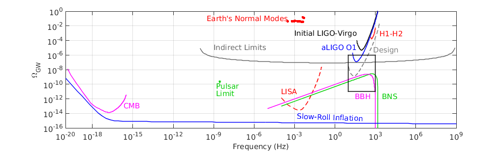
Figure 4 - 95% confidence region in average chirp mass - local rate plane
figure;
clf
%load contours
tmp=load('figure4_initial_BNS.dat');
M_init_n=tmp(:,1);
R_init_n=tmp(:,2);

tmp=load('figure4_initial_BBH.dat');
M_init_b=tmp(:,1);
R_init_b=tmp(:,2);

tmp=load('figure4_O1_BNS.dat');
M_O1_n=tmp(:,1);
R_O1_n=tmp(:,2);

tmp=load('figure4_O1_BBH.dat');
M_O1_b=tmp(:,1);
R_O1_b=tmp(:,2);

tmp=load('figure4_design_BNS.dat');
M_des_n=tmp(:,1);
R_des_n=tmp(:,2);

tmp=load('figure4_design_BBH.dat');
M_des_b=tmp(:,1);
R_des_b=tmp(:,2);


% set up plot

leg=zeros(1,3); % for legend


gg = axes;
set(gg,'FontSize',18);

% Initial LIGO-Virgo
leg(1)=loglog(M_init_n,R_init_n,'k','linewidth',2);
hold on
loglog(M_init_b,R_init_b,'k','linewidth',2);

% O1
leg(2)=loglog(M_O1_n,R_O1_n,'b-','linewidth',2);
loglog(M_O1_b,R_O1_b,'b-','linewidth',2);

% Design
leg(3)=loglog(M_des_n,R_des_n,'--','linewidth',2,'color',[0.5 0.5 0.5]);
loglog(M_des_b,R_des_b,'--','linewidth',2,'color',[0.5 0.5 0.5]);

% Add rectangle separating BNS from BBH
sep_rect=rectangle('Position',[2 1 0.5 1e7],'FaceColor',[0.8 0.8 0.8],'EdgeColor',[0.8,0.8,0.8]);
uistack(sep_rect,'bottom');

line([2 2+0.5],[1 1],'color','k')
line([2 2+0.5],[1e7 1e7],'color','k')

text(1.2,5,'BNS','fontsize',18)
text(4,5,'BBH','FontSize',18)


% CBC Limits

% flat-log distribution
rate_med=30;
rate_min=30+43;
rate_max=30-21;
mc_med=16.1;
mc_min=14.6;
mc_max=20;

plot([mc_med mc_med],[rate_min rate_max],'k','linewidth',2);
plot([mc_min mc_max],[rate_med rate_med],'k','linewidth',2);

text(17,9,'Flat','fontsize',15)

% power-law distribution
rate_med=99;
rate_min=99+138;
rate_max=99-70;
mc_med=8.6;
mc_min=5.7;
mc_max=11;

plot([mc_med mc_med],[rate_min rate_max],'k','linewidth',2);
plot([mc_min mc_max],[rate_med rate_med],'k','linewidth',2);

text(7,16,'Power','fontsize',15)


% Make Axes, etc

grid on
xlabel('M_c (M_{solar})','FontSize',18);
ylabel('R_{local} (Gpc^{-3} yr^{-1})','FontSize',18);
legend(leg,'Initial LIGO-VIRGO','aLIGO O1','Design')


axis([0 100 1 1e7])
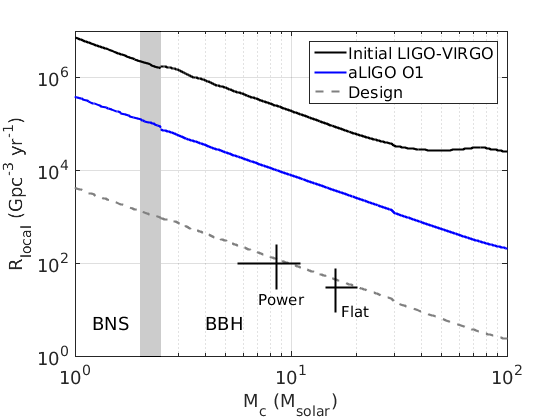
Figure 5 - Spectra from binary black holes for different mass distributions
% figure options
figure('units','normalized','position',[0 0 0.6 0.6]);

hh = axes;
fs1 = 18; %axis font size
fs2 = 18; %axis label font size
fs3 = 13; %legend font size
fs4 = 15; %label font size
lw=1; %linewidth for BBH spectra
set(hh,'FontSize',fs1)

leg=zeros(1,5);

% Flat log distribution
tmp=load('figure5_flatlog.dat');
freq=tmp(:,1);
omegaFlatMin=tmp(:,2);
omegaFlatMean=tmp(:,3);
omegaFlatMax=tmp(:,4);

% Poisson uncertainty band
cut = freq <= 1000 & freq>=10 & omegaFlatMin>0 & omegaFlatMax>0;
ff2 = freq(cut);
X_stat1a = [ff2; flipud(ff2)];
Y_stat1a = [omegaFlatMin(cut); flipud(omegaFlatMax(cut))];

leg(3) = loglog(freq,omegaFlatMean,'r-','linewidth',lw);
hold on


leg(4) = fill(X_stat1a, Y_stat1a, [1 0.8 0.8]);


% Power law distribution
tmp=load('figure5_powerlaw.dat');
freq=tmp(:,1);
omegaPowerMin=tmp(:,2);
omegaPowerMean=tmp(:,3);
omegaPowerMax=tmp(:,4);

% Poisson uncertainty band
cut = freq <= 1000 & freq>=10 & omegaPowerMin>0 & omegaPowerMax>0;
ff2 = freq(cut);
X_stat2a = [ff2; flipud(ff2)];
Y_stat2a = [omegaPowerMin(cut); flipud(omegaPowerMax(cut))];

leg(2)= fill(X_stat2a, Y_stat2a, [0.4 0.8 0.8]);
loglog(freq,omegaPowerMin,'-','linewidth',2,'Color', [0.4 0.8 0.8]);
loglog(freq,omegaPowerMax,'-','linewidth',2,'Color', [0.4 0.8 0.8]);
leg(1)= loglog(freq,omegaPowerMean,'color','g','linewidth',lw);


% Plot boundaries for flat log distribution
% (done here so that they lie on top of Poisson bands)
loglog(freq,omegaFlatMean,'r-','linewidth',lw);
loglog(freq,omegaFlatMin,'--','linewidth',2,'Color', [1 0.8 0.8]);
loglog(freq,omegaFlatMax,'--','linewidth',2,'Color', [1 0.8 0.8]);


% 3-Delta Distribution
tmp=load('figure5_3delta.dat');
freq=tmp(:,1);
omegatot=tmp(:,2);

leg(5)=loglog(freq,omegatot,'k-','linewidth',lw);


% PI Curves
% O1

tmp=load('PICurve_O1.dat');
freq=tmp(:,1);
Om=tmp(:,2);

loglog(freq,Om,'Color','b','LineStyle','-','linewidth',lw);
text(32,3e-7,'aLIGO O1','color','b','fontsize',fs4);

% Design

tmp=load('PICurve_design.dat');
freq=tmp(:,1);
Om=tmp(:,2);

loglog(freq,Om,'Color',[0.5 0.5 0.5],'LineStyle','--','linewidth',lw);
text(5.5e1,2e-8,'Design','color',[0.5,0.5,0.5],'FontSize',fs4);


% Legend and axes
ll=legend(leg,'Flat, Mean','Flat, Poisson','Power, Mean','Power, Poisson','3-Delta','Location','Northeast');
set(ll,'FontSize',fs3);


axis([10 1000 1e-11 1e-6])
xlabel('Frequency (Hz)','FontSize',fs1)
ylabel('\Omega_{GW}','FontSize',fs1)
grid on

grid minor

Supplement Figure 1 - Magnetic correlated noise budget
figure;
% Plot power-law fit to noise budget
% Omega(f) = A * (f/fref)^a with fref=1Hz
A=1.2e-8;
a=-0.9;

freq=[20 100];
Om=A*freq.^a;

loglog(freq,Om,'k','linewidth',2);
hold on

% Plot PI Curve
tmp=load('PICurve_O1.dat');
freq=tmp(:,1);
Om=tmp(:,2);
loglog(freq,Om,'k--');

% plotting options
grid on
set(gca,'fontsize',15);
xlabel('Frequency (Hz)','fontsize',15)
ylabel('\Omega_{\rm GW}','fontsize',15)
axis([20 100 1e-14 1])

legend('O1 PI Curve','Correlated Noise Budget','location','southwest')